Propagator formulation for transport processes
 Propagator in the wake of a cylinder for two selected points (diamonds). Dashed lines represent the velocity field, round points the origin of influence for the diamonds. The ellipses indicate the width of the Gaussian approximation.
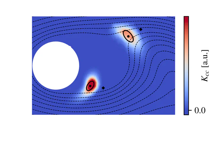
For linear transport equations
$$ \frac{\partial c}{\partial t} + \nabla\cdot c\boldsymbol{u} = \nabla\cdot D\nabla c $$ of some concentration $c(\boldsymbol{r}, t)$ (e.g., species or energy) subject to advection with a velocity field $\boldsymbol{u}(\boldsymbol{r}, t)$ and diffusion with strength $D(\boldsymbol{r}, t)$ , the future state after an arbitrarily long time step $\Delta t_{\textrm{prop}}$ needs to depend linearly on the field at $t$ , i.e., $$ c(\boldsymbol{r}, t + \Delta t_{\textrm{prop}} ) = \int d^3r' K_{\textrm{cc}} (\boldsymbol{r}, \boldsymbol{r}' ; \Delta t_{\textrm{prop}} , t) c(\boldsymbol{r}' , t). $$ $K_{\textrm{cc}}$ is called the propagator of the transport equation and is itself a solution of this equation with initial condition $K_{\textrm{cc}}(\boldsymbol{r}, \boldsymbol{r}' ; 0 , t) = \delta(\boldsymbol{r} - \boldsymbol{r}')$ for every $\boldsymbol{r}'$ . For a mesh with $N$ cells, one would have to solve $N$ PDEs to compute the propagator and store a field with $N^2$ values, which is computationally far too expensive. However, a much more efficient approximation is given by a shifted Gaussian $$ K_{\textrm{cc}} (\boldsymbol{r}, \boldsymbol{r}' ; \Delta t_{\textrm{prop}} , t) \propto \textrm{e}^{-1/2\big(\boldsymbol{r}' - \boldsymbol{r}^{\textrm{(or)}}\big)\boldsymbol{\Sigma}^{-1}\big(\boldsymbol{r}' - \boldsymbol{r}^{\textrm{(or)}}\big)}, $$ which can be calculated with little effort and does not require much memory.
For every point $\boldsymbol{r}$ in the domain, this operator advects the concentration value from its origin $\boldsymbol{r}^{\textrm{(or)}} (\boldsymbol{r}; \Delta t_{\textrm{prop}} , t)$ to $\boldsymbol{r}$ and diffuse with strength $\boldsymbol{\Sigma}(\boldsymbol{r}; \Delta t_{\textrm{prop}}, t)$ into an increasingly smeared out peak. Upon discretization, this amounts to cell-to-cell shifts with subsequent diffusion. Because very large time steps are permissible and the calculations are very simple, speed ups of several orders of magnitude compared to detailed CFD simulations are possible and brings us close to or even beyond real-time simulations.
Because this methodology relies on a priori knowledge of the velocity field, it is particularly suitable for recurrent flows (e.g., fluidized beds, bubble columns) or pseudosteady problems (e.g., moving beds).
References on propagator transport simulations (transport-based recurrence CFD and pseudosteady CFD-DEM):